Looking Through DeepVariant's Eyes- But In Your Browser
What happens when you take a CNN trained on ImageNet and point it at genomes? It works. Here's a browser tool where you can watch the whole thing happen.

Recently, I’ve been more involved with where and how deep learning meets genomics. Briefly tracing the history back, one of the first breakthroughs regarding this was DeepVariant, where variant calling task was being reframed as an image classification problem.
Back in the 2010s, the image classification task was the main “battleground” for the state-of-the-art algorithms, and this was where deep learning did bloom and made many breakthroughs long before the dawn of LLMs. And with the power of transfer learning, we were able to adapt them even to seemingly non-related fields like genomics, considering the sheer amount of data and pattern recognition powers the image classification models have gained.
DeepVariant was published by Google in 2017, and the core idea is almost too simple: instead of all that statistical machinery, what if you just turn the variant calling data into an image and ask a CNN? Not just any CNN; they took InceptionV3, a model that was trained on tens of thousands of images of golden retrievers, school buses, oyster mushrooms, and a thousand object classes. A model built for recognizing things in photographs, and they pointed it at genomes. And it worked better than the hand-engineered tools.
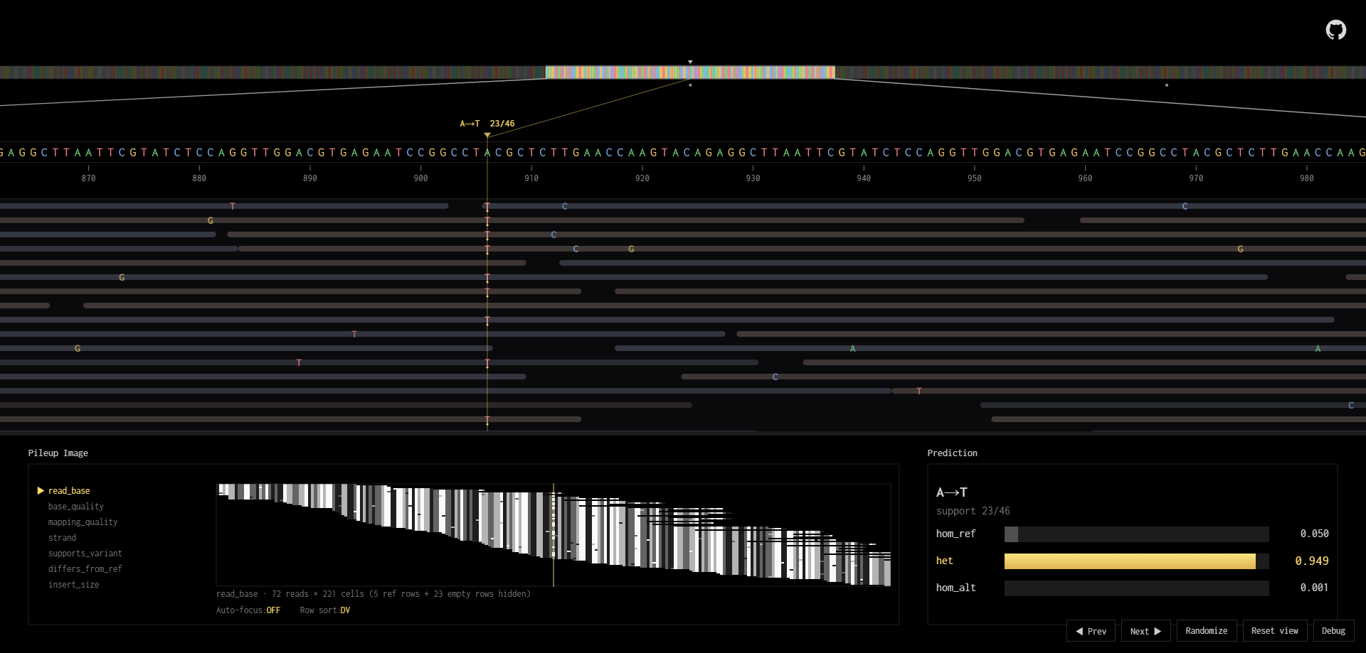
While exploring how the genomics information within the read “pileup” and the reference genome was represented as grayscale images, the official blog post “Looking Through DeepVariant’s Eyes” kept coming up. And after tinkering for a while, I had the urge to make a live version of it. So I rebuilt the pileup encoder, quantized the model, and wrapped a visualization around it. This effort resulted with this interactive toy-like genomics reader and pileup encoder tool that runs right in your browser, no data ever leaves the page.
You can visit the tool here: https://galinilin.github.io/deepvariant-tfjs/
For those who are interested in the details, let’s dive in.
What even is “variant calling”?
Variant calling is simply comparing a piece of a DNA sequence and a reference genome (with them being mapped with rigorous alignment tools), the “truth” set, and deciding if that piece of genome at a specific location has a variation or not. This lays the basics for how each individual’s genome does differ from the “average” human being.
Current DNA sequencing methods of ours aren’t able to generate precise information about the specific nucleic acids and their arrangements within the sample, they are mostly predictions (maybe super accurate predictions but still, predictions). They are keen to generate lots of errors and these error profiles differ from machine to machine. And essentially, variant calling is the work of filtering out the error that is produced by the sequencer machines in order to determine if that specific differentiation from reference is an error or a real variation within the analyzed sample.
Long before complex statistics analysis tools, this was mainly done by hand, by clinical variant specialists. Increasingly, tools like FreeBayes and GATK were being used for this task but it was mostly relying on hand-engineered parameters. And since different machines have different error profiles, if a new sequencing machine with a new method comes up, that error profile can be entirely different and you kind of have to start from scratch with your tuning.
DeepVariant took the famous InceptionV3 as backbone and generalized this variant calling task with representing each variant candidate as a set of 221x100 grayscale images. Each carries the information about the reads that the sequencer machine has outputted, the reference genome, prediction confidence scores and all and trained a 3-class multiclassifier system. Let’s inspect the details.
Representation and encoding of the pileup
As I’ve just mentioned, DeepVariant reframes this whole task as looking at 6 different grayscale images (7, depending on the version). Each candidate variant is being represented by an array of images sized as 221x100, and deciding whether the candidate we are looking at is a real heterozygous/homozygous variant, or there’s no variant at all; with their corresponding confidence outputs. The images are centered around the candidate variant location, seeing the neighboring bases 110bp-left and 110bp-right. Within each image; each row represents a read, and each column represents a genomic location. The representation images do encode specific information within that window like base read quality scores, read alignment confidence scores, reference base nucleic acid itself, read direction, and the network solely predicts on that.

Considering differentiations as variation candidates
Now as I mentioned earlier, sequencing machines can have slight errors from the actual data we are trying to probe. Not every position in the genome gets a pileup image built for it and fed to the network, that would be processing millions of images for a single analyzed sample. The candidate generation engine is the filter that decides which positions are even worth asking the model about.
The original implementation may vary slightly, but on our tool the logic within the candidate generation is pretty straightforward. First, a read only counts toward a candidate if it passes a minimum mapping quality (mapq >= 5), this value quantifies the confidence score of the aligner tool I mentioned earlier. And, for substitutions, a minimum read quality (base-Q >= 10) filter is applied. Then, for a position to actually become a candidate, it needs at least 2 reads supporting an alternate allele and those reads need to make up a minimum fraction of the total coverage at that column: 12% for SNVs, 6% for indels. These thresholds are intentionally permissive; the whole point is to let anything remotely plausible through and let the CNN make the real call. Even this most simplistic filtering can rule out significant non-candidates to be run against the CNN itself.
There’s also a second, stricter filter that kicks in when building the actual pileup image. Even if a position is flagged as a candidate, the reads that make it into the encoded image have to pass mapq >= 10 and base-Q >= 10. So the candidate generation casts a wide net, but the encoding stage is a bit pickier about what the model actually gets to see.
Adapting the encoded format to InceptionV3
Here’s the thing though: InceptionV3 was trained on 3-channel RGB real world images. DeepVariant feeds it 6 (or 7, depending on the version) channels. So how does that even work?
They didn’t do anything fancy like reshaping the channels or interleaving them into three. They just widened the very first convolutional layer’s kernel from (3, 3, 3, 32) to (3, 3, 6, 32) and let the model deal with it. The ImageNet-trained weights were copied into the first three channel slots, and channels 4 through 6 were randomly initialized. That one layer was the only modification. Everything else, all 23 million+ parameters across 70+ layers, is pure InceptionV3 with a 3-class softmax head on top.
This is what transfer learning actually looks like in practice. The first dozen or so layers of an ImageNet-trained CNN have already learned to detect edges, gradients, textures, spatial regularities; general-purpose visual features that stay useful whenever your input has any kind of spatial structure. The model doesn’t need to learn from scratch what an “edge” is or what “vertical alignment” looks like. It only needs to adapt its later layers to recognize the specific patterns that distinguish a real variant from sequencing noise. And that is exactly why you can take a model trained on golden retrievers and have it do clinical genomics.
Migration to the browser!
The released DeepVariant v1.8 WGS checkpoint is ~350 MB of TensorFlow checkpoint files, that’s not going to work for a browser tool. The conversion path was: restore the checkpoint in Keras, re-export through the tfjs converter to get a JavaScript-loadable layers model at 88 MB, then quantize the weights from float32 to uint8 which brings it down to 22 MB. That’s what the page actually downloads when you click “Launch Sandbox.”
Quantization always comes with a cost though, and you can’t just assume the model still works, you have to check. I ran cross-runtime parity tests against the original Python model, and the float32 tfjs version matched Python within float32 epsilon (max difference around 2.38e-7). The uint8 quantized version shifts softmax probabilities by under 2%, and the argmax -meaning the actual predicted class- is preserved on every test input. Good enough for a demonstration tool.
One porting issue that took me a while to track down: DeepVariant’s Keras model includes a Lambda layer that does input preprocessing; normalizing the raw [0, 254] pixel intensities into the range [-1, 1]. tfjs can’t serialize Lambda layers because the Python function inside them is a black box to the JavaScript runtime. So that preprocessing had to be lifted out and done manually in TypeScript before passing the tensor to the model. Without it, the model returns complete nonsense. With it, predictions match Python results exactly.
I’ve been doing deep learning since 2017 and over the last year I’ve been gravitating more towards where it meets biology. Protein folding breakthroughs and the protein language models drew me in first, then variant calling, and then the broader landscape of genomic foundation models. DeepVariant felt like the cleanest place to start; a CNN doing real, useful work in real clinical pipelines, with a paper trail you can actually sit down and read.
Building this thing made a few things concrete for me. Transfer learning is quietly the most important idea in applied deep learning. Although self-supervised pretraining approaches have given promising results on building base models recently; most interesting domains, biology included, will never have like ImageNet-scale labeled data. The whole game is finding a backbone that already knows enough and adapting it carefully. DeepVariant does this by changing exactly one layer, and I find that kind of beautiful.
And models you can poke at are models you actually understand. Reading the paper taught me architecture. Sliding a low-quality variant into the predict window and watching the softmax bars refuse to commit taught me what the model actually does. That’s why I built the sandbox, and that’s how I actually learned what was going on inside those 24 million parameters.
Until next time, much love.